
In this paper we will provide a step by step guide on how to install a single-instance of OpenTSDB using the latest versions of the underlying technology, Hadoop and HBase. We will also provide some background on the state of existing monitoring solutions.
Table of contents
- Abstract
- Background
- The monitoring revolution
- Setting up a single node OpenTSDB instance on Debian 7 Wheezy
- Installing OpenTSDB
- Feeding data into OpenTSDB
- Performance comparison
Background
Since its inception in 1999 rrdtool (the underlying storage mechanism of once universal MRTG) has been the base of many popular monitoring solutions; Cacti, collectd, Ganglia, Munin, Observium, OpenNMS and Zenoss, to name a few.
There are a number of problems with the current approach and we will highlight some of these here.
Please note that this includes Graphite and its backend Whisper, which is based on the same basic design as rrdtool and has some of the same limitations.
Performance problems - Welcome to I/O-hell
When MRTG and rrdtool was created the preservation of disk space was more important than preservation of disk operations and the default collection interval was 5 minutes (which many are still using). The way rrdtool is designed it requires quite a few random reads and writes per datapoint. It also re-reads, computes the average, and writes old data again according to the RRA rules defined which causes additional I/O load. In 2014 memory is cheap, disk storage is cheap and CPU is fairly cheap. Disk I/O operations (IOPS) however are still very expensive in terms of hardware. The recent maturing of SSD provides extreme amounts of IOPS for a reasonable price, but the drive sizes are fractional. The result is that in order to scale IOPS-wise you currently need many low-space SSDs to get the required space, or many low-IOPS spindle drives to get the required IOPS:
Samsung EVO 840 1TB SSD - 98.000 IOPS - 470 USD
Seagate Barracuda 3TB - 240 IOPS - 110 USD
You would need $44.880 (408 drives) worth of spindle drives in order to match a single SSD drive in terms of I/O-performance. On the other hand a $2.000 array of spindle drives would get you a net ~54 TB of space. The cost of SSD to reach the same volume would be $25.380. Not to mention the cost of servers, power, provisioning, etc.
Note: This is the cheapest available bulk consumer drives and comparable OEM drives (SSD, spindle) for a HP server will be 6 to 30 times more expensive.
In rrdtool version 1.4, released in 2009, rrdcached was introduced as a caching daemon for buffering multiple data updates and reducing the number of random I/O operations by writing several related datapoints in sequence. It took a couple of years before this new feature was implemented in most of the common open source monitoring solutions.
For a good introduction into the internals of rrdtool/rrdcached updates and the problems with I/O scaling look at presentation by Sebastian Harl, How to Escape the I/O Hell
Scaling problems
Most of today’s monitoring systems do not easily scale-out. Scale-out, or scaling horizontally, is when you can add new nodes in response to increased load. Scaling up by replacing existing hardware with state-of-the-art hardware is both expensive and only buys you limited time before the next even more expensive necessary hardware upgrade. Many systems offer distributed polling but none offer the option of spreading out the disk load. For example; you can scale Zenozz for High Availability but not performance.
Loss of detail
Current RRD based systems will aggregate old data into averages in order to save storage space. Most technicians do not have the in depth knowledge in order to tune the rules for aggregation and will leave the default values as is. Using cacti as an example and looking at the cacti documentation we see that in a very short time, 2 months, data is averaged to a single data point PER DAY. For systems such as Internet backbones where traffic vary a lot from bottom (30% utilization for example) to peak (90% utilization for example) during a day only the average of 60% is shown in the graphs. This in turn makes troubleshooting by comparing old data difficult. It makes trending based on peaks/bottoms impossible and it may also lead to wrong or delayed strategic decisions on where to invest in added capacity.
Lack of flexibility
In order to collect, store and graph new kinds of metrics an operator would need a certain level of programming skills and experience with the internals of the monitoring system. Adding new metrics to the systems would range from hours to weeks depending on the skill and experience of the operator. Creating new graphs based on existing metrics is also very difficult on most systems. And not within reach for the average operator.
The monitoring revolution
We are currently at the beginning of a monitoring revolution. The advent of cloud computing and big data has created a need for measuring lots of metrics for thousands of machines at small intervals. This has sparked the creation of completely new monitoring components. One of the components where we now have improved alternatives is for efficient metric storage.
The first is OpenTSDB, a “Scalable, Distributed, Time Series Database” that begun development at StumbleUpon in 2011 and aimed at solving some of the problems with existing monitoring systems. OpenTSDB is built in top of Apache HBase which is a scalable and performant database that builds on top of Apache Hadoop. Hadoop is a series of tools for building large and scalable distributed systems. Back in 2010 Facebook already had 2000 machines in a Hadoop cluster with 21PB (that is 21.000.000 GB) of combined storage.
The second is an interesting newcommer, InfluxDB, that began development in 2013 and has the goal of offering scalability and performance without the requirements of HBase/Hadoop.
In addition to advances in performance these alternatives also decouple storage of metrics and display of graphs and abstract the interaction in simple and well-defined APIs. This makes it easy for developers to create improved frontends rapidly and this has already resulted in several very attractive open-source frontends such as Metrilyx (OpenTSDB), Grafana (InfluxDB, Graphite, soon OpenTSDB), StatusWolf (OpenTSDB), Influga (InfluxDB).
Setting up a single node OpenTSDB instance on Debian 7 Wheezy
In the rest of this paper we will set up a single node OpenTSDB instance. OpenTSDB builds on top of HBase and Hadoop and scales to very large setups easily. But it also delivers substantial performance on a single node which is deployed in less than an hour. There are plenty of guides on installing a Hadoop cluster but here we will focus on the natural first step of getting a single node running using recent releases of the relevant software:
- OpenTSDB 2.0.0 - Released 2014-05-05
- HBase 0.98.2 - Released 2014-05-01
- Hadoop 2.4.0 - Released 2014-04-07
If you later require to deploy a larger cluster consider using a framework such as Cloudera CDH or Hortonworks HDP which are open-source platforms which package Apache Hadoop components and provides a fully tested environment and easy-to-use graphical frontends for configuration and management. It is recommended to have at least 5 machines in a HBase cluster supporting OpenTSDB.
This guide assumes you are somewhat familiar with using a Linux shell/command prompt.
Hardware requirements
- CPU cores: Max (Limit to 50% of your available CPU resources)
- RAM: Min 16 GB
- Disk 1 - OS: 10 GB - Thin provisioned
- Disk 2 - Data: 100 GB - Thin provisioned
Operating system requirements
This guide is based on a recently installed Debian 7 Wheezy 64bit installed without any extra packages. See the official documentation for more information.
All commands are entered as root user unless otherwise noted.
Pre-setup preparations
We start by installing a few tools that we will need later.
apt-get install wget make gcc g++ cmake maven
Create a new ext3 partition on the data disk /dev/sdb:
(echo "n"; echo "p"; echo ""; echo ""; echo ""; echo "t"; echo "83"; echo "w") | fdisk /dev/sdb

mkfs.ext3 /dev/sdb1
ext3 is the recommended filesystem for Hadoop.
Create a mountpoint /mnt/data1 and add it to the file system table and mount the disk:
mkdir /mnt/data1
echo "/dev/sdb1     /mnt/data1    ext3    auto,noexec,noatime,nodiratime   0   1" | tee -a /etc/fstab
mount /mnt/data1
Using noexec for the data partition will increase security as nothing on the data partition will be allowed to ever execute.
Using noatime and nodiratime increases performance since the read access timestamps are not updated on every file access.
Installing java from packages
Installing java on Linux can be quite challenging due to licensing issues, but thanks to the guys over at Launchpad.net who are providing a repository with a custom java package this can now be done quite easy.
We start by adding the launchpad java repository to our /etc/apt/sources.list file:
echo "deb http://ppa.launchpad.net/webupd8team/java/ubuntu precise main" | tee -a /etc/apt/sources.list
echo "deb-src http://ppa.launchpad.net/webupd8team/java/ubuntu precise main" | tee -a /etc/apt/sources.list
Add the signing key and download information from the new repository:
apt-key adv --keyserver hkp://keyserver.ubuntu.com:80 --recv-keys EEA14886
apt-get update
Run the java installer:
apt-get install oracle-java7-installer
Follow the instructions on screen to complete the Java 7 installation.
Installing HBase
OpenTSDB has its own HBase installation tutorial here. It is very brief and does not use the latest versions or snappy compression.
Download and unpack HBase:
cd /opt
wget http://apache.vianett.no/hbase/hbase-0.98.2/hbase-0.98.2-hadoop2-bin.tar.gz
tar xvfz hbase-0.98.2-hadoop2-bin.tar.gz
export HBASEDIR=`pwd`/hbase-0.98.2-hadoop2/
Increase the system-wide limitations of open files and processes from the default of 1000 to 32000 by adding a few lines to /etc/security/limits.conf:
echo "root    -               nofile  32768" | tee -a /etc/security/limits.conf
echo "root    soft/hard       nproc   32000" | tee -a /etc/security/limits.conf
echo "*    -               nofile  32768" | tee -a /etc/security/limits.conf
echo "*    soft/hard       nproc   32000" | tee -a /etc/security/limits.conf
The settings above will only take effect if we also add a line to /etc/pam.d/common-session:
echo "session required pam_limits.so" | tee -a /etc/pam.d/common-session
Install snappy
Snappy is a compression algorithm that values speed over compression ratio and this makes it a good choice for high throughput applications such as Hadoop/HBase. Due to licensing issues Snappy does not ship with HBase and need to be installed on top.
The installation process is a bit complicated and has caused headache for many people (me included). Here we will show a method of installing snappy and getting it to work with the latest version of HBase and Hadoop.
Compression algorithms in HBase Compression is the method of reducing the size of a file or text without losing any of the contents. There are many compression algorithms available and some focus on being able to create the smallest compressed file at the cost of time and CPU usage while other achieve reasonable compression ratio while being very fast.
Out of the box HBase supports gz(gzip/zlib), snappy and lzo. Only gz is included due to licensing issues. Unfortunately gz is a slow and costly algorithm compared to snappy and lzo. In a test performed by Yahoo (see slides here, page 8) gz achieves 64% compression in 32 seconds. lzo 47% in 4.8 seconds and snappy 42% in 4.0 seconds. lz4 is another protocol considered for inclusion that is even faster (2.4 seconds) but requires much more memory.
For more information look at the Apache HBase Handbook - Appendix C - Compression
Building native libhadoop and libsnappy
In order to use compression we need the common Hadoop library, libhadoop.so, and the snappy library, libsnappy.so. HBase ships without libhadoop.so and the libhadoop.so that ships in the Hadoop Package is only for 32 bit OS. So we need to compile these files ourself.
Start by downloading and installing ProtoBuf. Hadoop requres version 2.5+ which is not available as a Debian package unfortunately.
wget --no-check-certificate https://protobuf.googlecode.com/files/protobuf-2.5.0.tar.gz
tar zxvf protobuf-2.5.0.tar.gz
cd protobuf-2.5.0
./configure; make; make install
export LD_LIBRARY_PATH=/usr/local/lib/
Download and compile Hadoop:
apt-get install zlib1g-dev
wget http://apache.uib.no/hadoop/common/hadoop-2.4.0/hadoop-2.4.0-src.tar.gz
tar zxvf hadoop-2.4.0-src.tar.gz
cd hadoop-2.4.0-src/hadoop-common-project/
mvn package -Pdist,native -Dskiptests -Dtar -Drequire.snappy -DskipTests
Copy the newly compiled native libhadoop library into /usr/local/lib, then create the folder in which HBase looks for it and create a shortcut from there to /usr/local/lib/libhadoop.so:
cp hadoop-common/target/native/target/usr/local/lib/libhadoop.* /usr/local/lib
mkdir -p $HBASEDIR/lib/native/Linux-amd64-64/
cd $HBASEDIR/lib/native/Linux-amd64-64/
ln -s /usr/local/lib/libhadoop.so* .
Install snappy from Debian packages:
apt-get install libsnappy-dev
Configuring HBase
Now we need to do some basic configuration before we can start HBase. The configuration files are in $HBASEDIR/conf/.
conf/hbase-env.sh
A shell script setting various environment variables related to how HBase and Java should behave. The file contains a lot of options and they are all documented by comments so feel free to look around in it.
Start by setting the JAVA_HOME, which points to where Java is installed:
export JAVA_HOME=/usr/lib/jvm/java-7-oracle/
Then increase the size of the Java Heap from the default of 1000 which is a bit low:
export HBASE_HEAPSIZE=8000
conf/hbase-site.xml
An XML file containing HBase specific configuration parameters.
<configuration>

   <property>
    <name>hbase.rootdir</name>
    <value>/mnt/data1/hbase</value>
  </property>

  <property>
    <name>hbase.zookeeper.property.dataDir</name>
    <value>/mnt/data1/zookeeper</value>
  </property>

</configuration>
Testing HBase and compression
Now that we have installed snappy and configured HBase we can verify that HBase is working and that the compression is loaded by doing:
$HBASEDIR/bin/hbase org.apache.hadoop.hbase.util.CompressionTest /tmp/test.txt snappy
This should output some lines with information and end with SUCCESS.
Starting HBase
HBase ships with scripts for starting and stopping it, namely start-hbase.sh and stop-hbase.sh. You start HBase with
$HBASEDIR/bin/start-hbase.sh
Then look at the log to ensure it has started without any serious errors:
tail -fn100 $HBASEDIR/bin/../logs/hbase-root-master-opentsdb.log
If you want HBase to start automatically on boot you can use a process management tool such as Monit or simply put it in /etc/rc.local:
/opt/hbase-0.98.2-hadoop2/bin/start-hbase.sh
Installing OpenTSDB
Start by installing gnuplot, which is used by the native webui to draw graphs:
apt-get install gnuplot
Then download and install OpenTSDB:
wget https://github.com/OpenTSDB/opentsdb/releases/download/v2.0.0/opentsdb-2.0.0_all.deb
dpkg -i opentsdb-2.0.0_all.deb
Configuring OpenTSDB
The configuration file is /etc/opentsdb/opentsdb.conf. It has some of the basic configuration parameters but not nearly all of them. Here is the official documentation with all configuration parameters.
The defaults are reasonable but we need to make a few tweaks, the first is to add this:
tsd.core.auto_create_metrics = true
This will make OpenTSDB accept previously unseen metrics and add them to the database. This is very useful in the beginning when feeding data into OpenTSDB. Without this you will have to use the command mkmetric for each metric you will store and get errors that might be hard to trace if the metric you create do not match what is actually sent.
Then we will add support for chunked requests via the HTTP API:
tsd.http.request.enable_chunked = true
tsd.http.request.max_chunk = 16000
Some tools and plugins (such as our own improved collectd to OpenTSDB plugin) send multiple data points in a single HTTP request for increased efficiency and requires this setting to be enabled.
Creating HBase tables
Before we start OpenTSDB we need to create the necessary tables in HBase:
env COMPRESSION=SNAPPY HBASE_HOME=$HBASEDIR /usr/share/opentsdb/tools/create_table.sh
Starting OpenTSDB
Since version 2.0.0 OpenTSDB ships as a Debian package and includes SysV init scripts. To start OpenTSDB as a daemon running in the background we run:
service opentsdb start
And then check the logs for any errors or other relevant information:
tail -f /var/log/opentsdb/opentsdb.log
If the server is started successfully the last line of the log should say:
13:42:30.900 INFO [TSDMain.main] - Ready to serve on /0.0.0.0:4242
And you can now browse to your new OpenTSDB in a browser using http://hostname:4242 !
Feeding data into OpenTSDB
It is not within the scope of this paper to go into details about how to feed data into OpenTSDB but we will give a quick introduction here to get you started.
A note on metric naming in OpenTSDB
Each datapoint has a metric name such as df.bytes.free and one or more tags such as host=server1 and mount=/mnt/data1. This is closer to the proposed Metrics 2.0 standard for naming metrics than the traditional naming of df.bytes.free.server1.mnt-data. This makes it possible to create aggregates across tags and combine data easily using the tags.
OpenTSDB stores each datapoint with a given metric and tags in one HBase row per hour. But due to a HBase issue it still has to scan every row that matches the metric, ignoring the tags. Even though it will only return the data also matching the tags. This results in very much data being read and it will be very slow to read if there is a large number of data points for a given metric. The default for the collectd-opentsdb plugin is to use the read plugin name as metric, and other values as tags. In my case this results in 72.000.000 datapoints per hour for this metric. When generating a graph all of this data has to be read and evaluated before drawing a graph. 24 hours of data is over 1.7 billion datapoints for this single metric and results in a read performance of 5-15 minutes for a simple graph.
A solution to this is to use shift-to-metric, as mentioned in the OpenTSDB user guide. Shift-to-metric is simply moving one or more data identifiers from tags to the metric in order to reduce the cardinality (number of values) for a metric, and hence the time required to read out the data we want. We have modified the collectd-opentsdb java plugin in order to shift the tags to metrics, and this increases read-performance by ~1000x down to 10-100ms. Read the section about collectd below for more information on our modified plugin.
tcollector
tcollector is the default agent for collecting and sending data from a Linux server to a OpenTSDB server. It is based on Python and plugins / addons can be written in any language. It ships with the most common plugins to collect information about disk usage and performance, cpu and memory statistics and also for some specific systems such as mysql, mongodb, riak, varnish, postgresql and others. tcollector is very lightweight and features advanced de-duplication in order to reduce unneeded network traffic.
The commands for installing dependencies and downloading tcollector are
aptitude install git python
cd /opt
git clone git://github.com/OpenTSDB/tcollector.git
Configuration is in the startup script tcollector/startstop, you will need to uncomment and set the value of TSD_HOST to point to your OpenTSDB server.
To start it run
/opt/tcollector/startstop start
This is also the command you want to add to /etc/rc.local in order to have the agent automatically start at boot. Logfiles are saved in /var/log/tcollector.log and they are rotated automatically.
peritus-tc-tools
We have developed a set of tcollector plugins for collecting statistics from
- ISC DHCPd server, about number of DHCP events and DHCP pool sizes
- OpenSIPS, total number of subscribers and registered user agents
- Atmail, number of users, admins, sent and received emails, logins and errors
As well as a high performance replacement for smokeping called tc-ping.
These plugins are available for download from our GitHub page.
collectd-opentsdb
collectd is the system statistics collection daemon and is a widely used system for collecting metrics from various sources. There are several options for sending data from collectd to OpenTSDB but one way that works well is to use the collectd-opentsdb java write plugin.
Since collectd is a generic metric collection tool the original collectd-opentsdb plugin will use the plugin name (such as snmp) as the metric, and use tags such as host=servername, plugin_instance=ifHcInOctets and type_instance=FastEthernet0/1.
As mentioned in the note on metric naming in OpenTSDB this can be very inefficient when data needs to be read again resulting in read performance potentially thousands of times slower than optimal (<100ms). To alleviate this we have modified the original collectd-opentsdb plugin to store all metadata as part of the metric. This gives metric names such as ifHCInBroadcastPkts.sw01.GigabitEthernet0 and very good read performance.
The modified collectd-opentsdb plugin can be downloaded from our GitHub repository.
Monitoring OpenTSDB
To monitor OpenTSDB itself install tcollector as described above on the OpenTSDB server and set TSD_HOST to localhost in /opt/tcollector/startstop.
You can then go to http://opentsdb-server:4242/#start=1h-ago&end=1s-ago&m=sum:rate:tsd.rpc.received%7Btype=*%7D&o=&yrange=%5B0:%5D&wxh=1200x600 to view a graph of amount of data received in the last hour.
Performance comparison
Lastly we include a little performance comparison between the latest version of OpenTSDB+HBase+Hadoop, a previous version of OpenTSDB+HBase+Hadoop that we have used for a while as well as rrdcached which ran in production for 4 years at a client.
The workload is gathering and storing metrics from 150 Cisco switches with 8200 ports/interfaces every 5 seconds. This equals about 15.000 points per second.
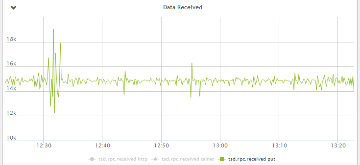
Figure 1 - Data received by OpenTSDB per second
Collection
Even though it is not the primary focus, we include some data about collection performance for completeness. Collection is done using the latest version of collectd and the builtin SNMP plugin.
NB #1: There is a memory leak in the way collectd’s SNMP plugin uses the underlying libsnmp library and you might need to schedule a restart of the collectd service as a workaround for that if handling large workloads.
NB #2: Due to limitations in the libnetsnmp library you will run into problems if polling many (1000+) devices with a single collectd instance. A workaround is to run multiple collectd instances with fewer hosts.
Figure 2 shows that collection through SNMP polling consumes about 2200Mhz. We optimized some of the data types and definitions in collectd when moving to OpenTSDB and achieved a 20% performance increase in the polling as seen in Figure 3.
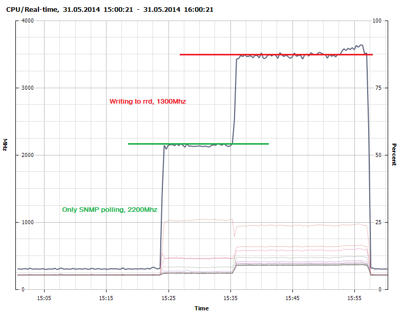
Figure 2 - CPU Usage - SNMP polling and writing to RRDcached
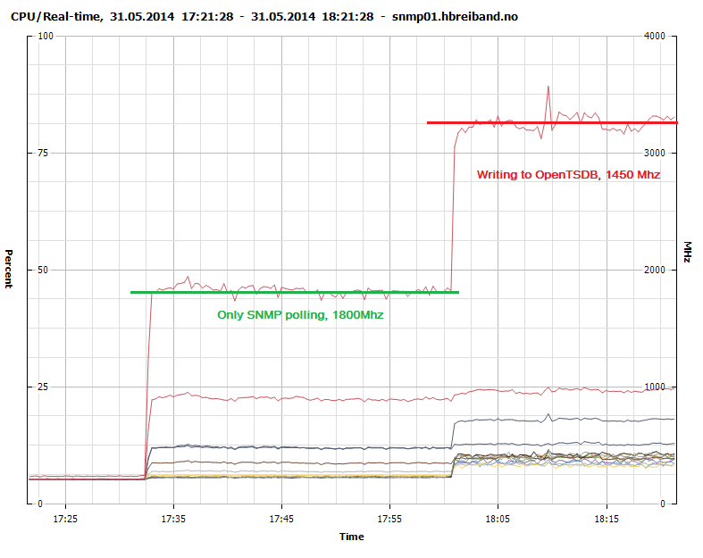
Figure 3 - CPU Usage - SNMP polling and sending to OpenTSDB
Writing to the native rrdcached write plugin consumes 1300Mhz while our modified collectd-opentsdb plugin consumes 1450Mhz. It is probably possible to create a much more efficient write plugin with more advanced knowledge of concurrency and using a lower level language such as C.
Storage
When considering storage performance we will look at CPU usage and disk IOPS since these are the primary drivers of cost in today’s datacenters.
collectd + rrdcached
CPU usage - 1300Mhz, see Figure 2 above.
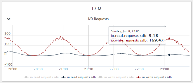
Figure 4 - Disk write IOPS - Fluctuating between 10 and 170 IOPS during the 1 hour flush period.
OpenTSDB + Hbase 0.96 + Hadoop 1
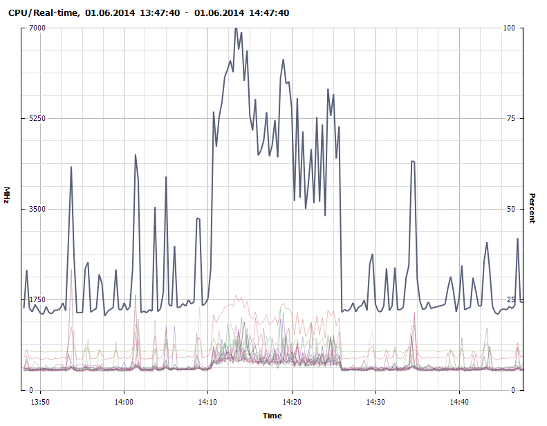
Figure 5 - CPU usage - 1700Mhz baseline with peaks of 7000Mhz during Java Garbage Collection (GC) (untuned).
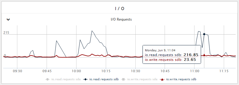
Figure 6 - Disk write IOPS - 5 IOPS average with peaks of 25 IOPS during Java GC. We also see that disk read IOPS are much higher and this is due to regular compaction of the database and can be tuned. Reads in general can be reduced by increasing caching with more RAM if necessary.
OpenTSDB + HBase 0.98 + Hadoop 2

Figure 7 - CPU usage - 1200Mhz baseline with peaks of 5000-6000Mhz during Java GC (untuned).
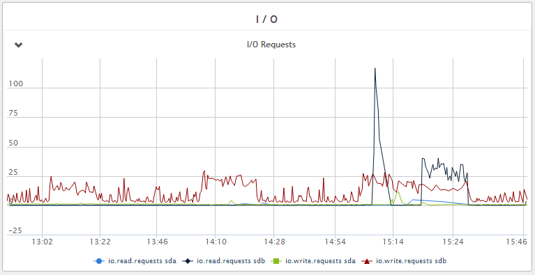
Figure 8 - Disk write IOPS - < 5 IOPS average with peaks of 25 IOPS during Java GC. Much less read IOPS during compaction compared to HBase 0.96.
Conclusion
Even without tuning, a single instance OpenTSDB installation is able to handle significant amounts of data before running into IO problems. This comes at a cost of CPU, currently OpenTSDB will consume > 300% the amount of CPU cycles compared to rrdcached for storage. But this is offset by a 85-95% reduction in disk load. In absolute terms for our particular set up (one 2 year old HP DL360p Gen8 running VMware vSphere 5.5) CPU usage increased from 15% to 25% while reducing IOPS load from 70% to < 10%.
Fine tuning of parameters (such as Java GC) as well as detailed analysis of memory usage is outside the scope of this brief paper and detailed information may be found elsewhere (51,52,53) for those interested.
Stian Ovrevage

Stian is a senior consultant and founder at Peritus Consulting AS. He is currently managing the technical systems for a small FTTH ISP in Norway. He also does consulting for other clients when time permits. When not digging deep into technical challenges he enjoys the outdoors.
Also on [GitHub][59], [LinkedIn][58], [Facebook][56], [Google+][57] and [Twitter][55].
Peritus Consulting Technical Reports

Technical reports are in-depth articles aimed at giving actionable advice on new technologies as well as recommended best practices based on tried and true solutions. We cover areas that are lacking of good in depth coverage online but will not re-write topics that are already covered in a satisfactory way elsewhere. We also write tech notes which are shorter pieces with thoughts and tips on both technology and the way technology should be used optimally. Our official webpage (in Norwegian) is at [www.peritusconsulting.no][60], articles are published on our [GitHub Page][61], we are also on [Twitter][62], [LinkedIn][64] and [Facebook][63].